This post summarizes my work during week 5-6 of my summer internship.

I finished the training of the model mentioned in the last report. The result was disappointing. Then I modified the model and got a fairly good result. For convenience, I will mention the model mentioned in the last report as Model I, and the modified model as Model II and Model III.

All the training curves and visualization images are created with Tensorboard Toolkit ([1]).

You can get a PDF version of this post from here.

The source code of DL Background Subtraction is available on my Github.

Contents

• Part I First experiment
  • 1.1 Hardware configuration
  • 1.2 Hyperparameters
  • 1.3 Experiment result
    • 1.3.1 Training curve
    • 1.3.2 Image visualization
• Part II Modification of the model
• Part III experiment result of the modified models
  • 3.1 Training curve
  • 3.2 Checkboard artifacts
  • 3.3 Comparison with classical methods

Part I First experiment

The first experiment is based on Model I. Refer to figure 1.1 as a review of the model.

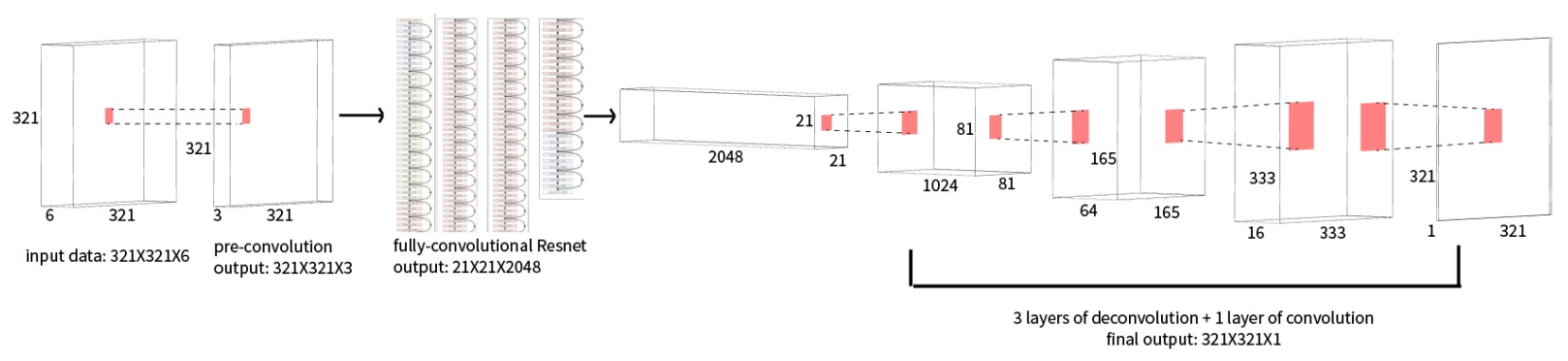
Figure 1.1 the model proposed in the last report

1.1 Hardware configuration

As is mentioned in the last report, I use cloud server to run the code. The hardware information is shown in the following table.

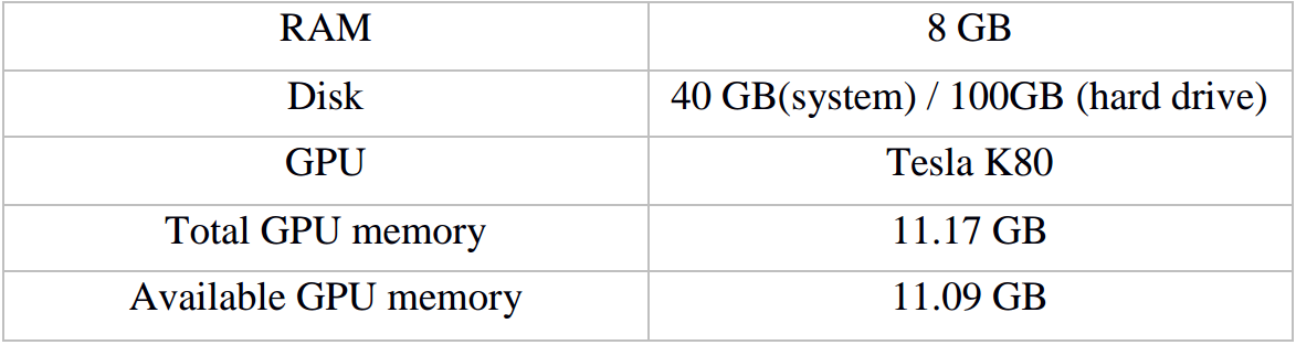
Table 1.1 Hardware configuration

1.2 Hyperparameters

In the last report, I mentioned the value of some hyper-parameters, but I modify some of them in my actual experiment. The following results are all based on the new set of parameters. Refer to table 1.2.

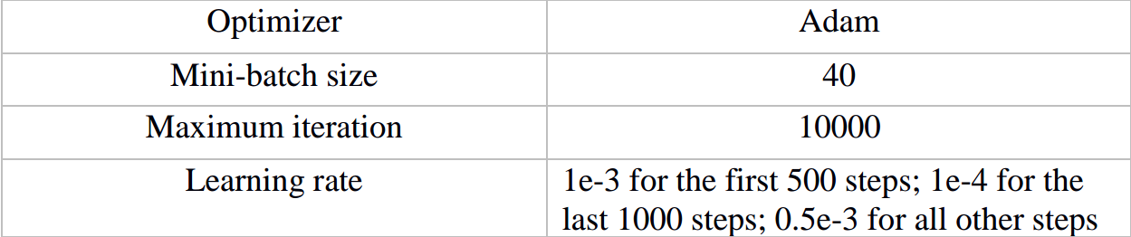
Table 1.2 value of hyperparameters

1.3 Experiment result

1.3.1 Training curve

Figure 1.2 shows part of the training curve (from step 5000 to the end).

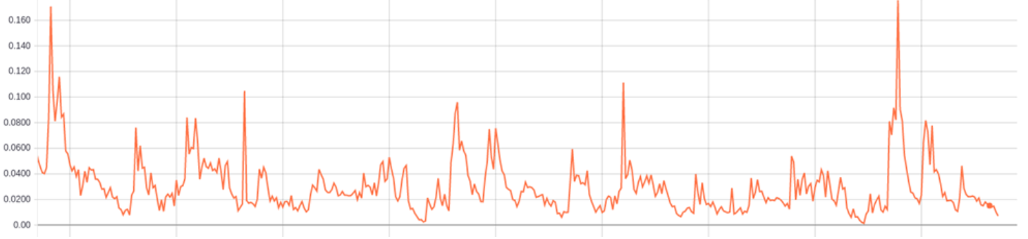
Figure 1.2 training curve of Model I (from step 5000 to the end)

It is clear that the cross-entropy loss on training set keeps vibrating within a relatively large range. This result is far from satisfactory. And it is not surprising that the loss on the test set is as high as 0.167.

1.3.2 Image visualization

I select one frame from test set and visualize the output feature map of each layer. Refer to figure 1.3.

In the output feature map of sigmoid activation, the activated region is approximately the same as ground truth, which means that the training does work. But after 10000 steps of iteration, the crossentropy loss is still vibrating on the training set and remains pretty high on the test set. Based on these analyses, we can come to the conclusion that the training samples are too few for the loss function to converge to the global minimum. Therefore, parameter-reduction is needed.

There is another interesting characteristic. Each feature map in figure 1.3 has checkboard artifacts. This is due to deconvolutional operations. (In deconvolutional layer, when stride is not 1, zeros will be filled into feature map. Refer to [2]) This will also be improved in the new models.

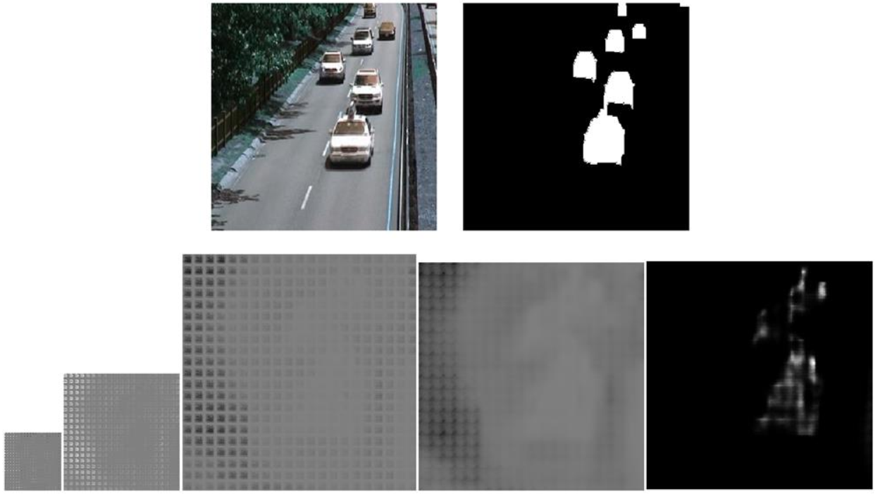
Figure 1.3 (Model I) visualization result of one frame in test set; for each feature map, only the first channel is shown. Top: original image and ground truth; Bottom, from left to right: the output feature of three deconvolutional layers, one convolution layer, and the final sigmoid activation

Part II Modification of the model

For the convenience of comparison, the architecture of Model I is recorded in detail. Refer to table 1.3. (Pay attention to the horrible amount of parameters). Table 1.4 and 1.5 shows the architecture details of Model II and III respectively. The number of parameters is reduced to a large degree in both models.

• Model II differs from Model I in the following two aspects.

1. Use 3D average pooling to reduce the output feature map of ResNet.
2. Use additional max pooling layers.
3. Use smaller deconvolutional filters to reduce the number of parameters.
   • Model III does not have additional max pooling layers. Instead, I use larger deconvolutional filters.

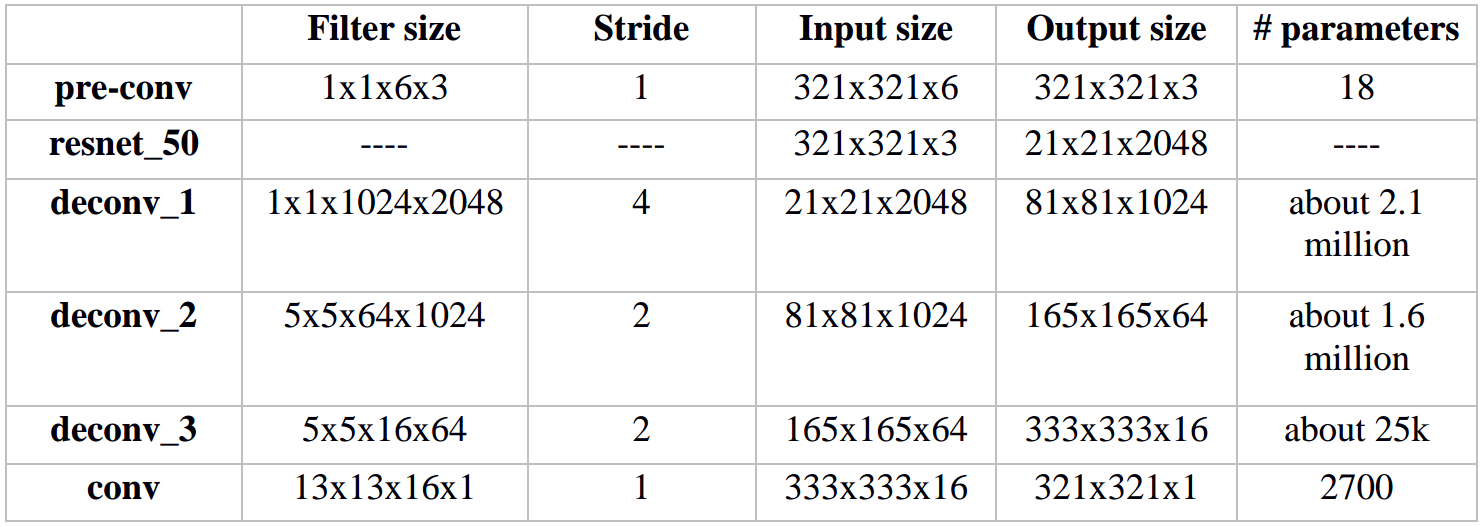
Table 2.1 architecture details of Model I

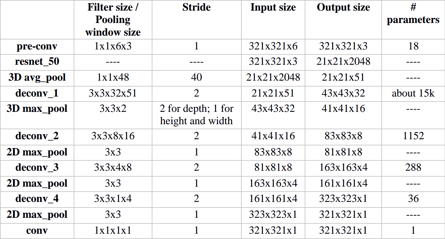
Table 2.2 architecture details of Model II

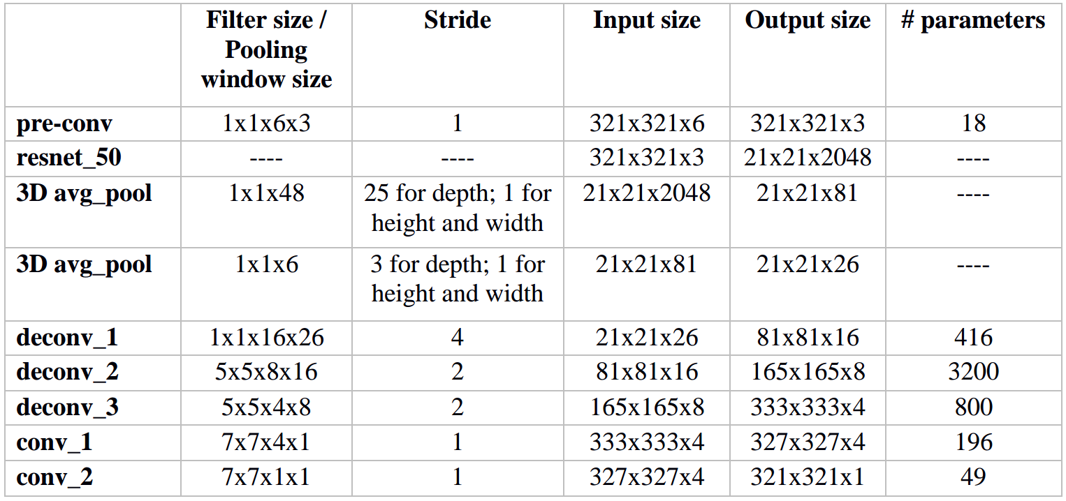
Table 2.3 architecture details of Model III

It is worth noting that Model II and III use different methods to improve checkboard artifacts. In Model II, additional max pooling layers eliminate extra zeros in the deconvolutional feature map. In Model III, larger deconvolutional filters can cover more non-zero elements. I will compare them in the following sections.

Part III experiment result of the modified models

3.1 Training curve

It took about 2 days 10 hours to train each model. Figure 3.1 and 3.2 show training curve of Model II and Model III respectively. Compared to Model I, both II and III converge fairly well.

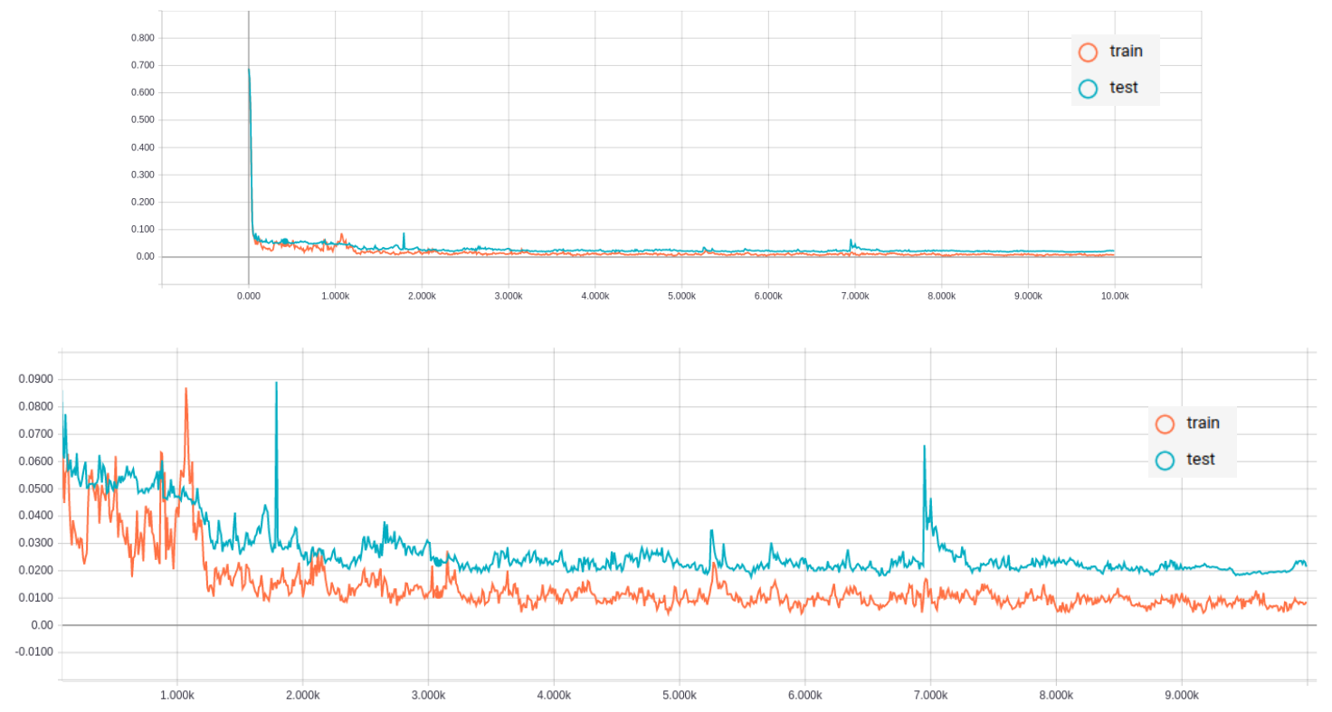
Figure 3.1 Training curve of Model II
Top: training curve; Bottom: zoom in

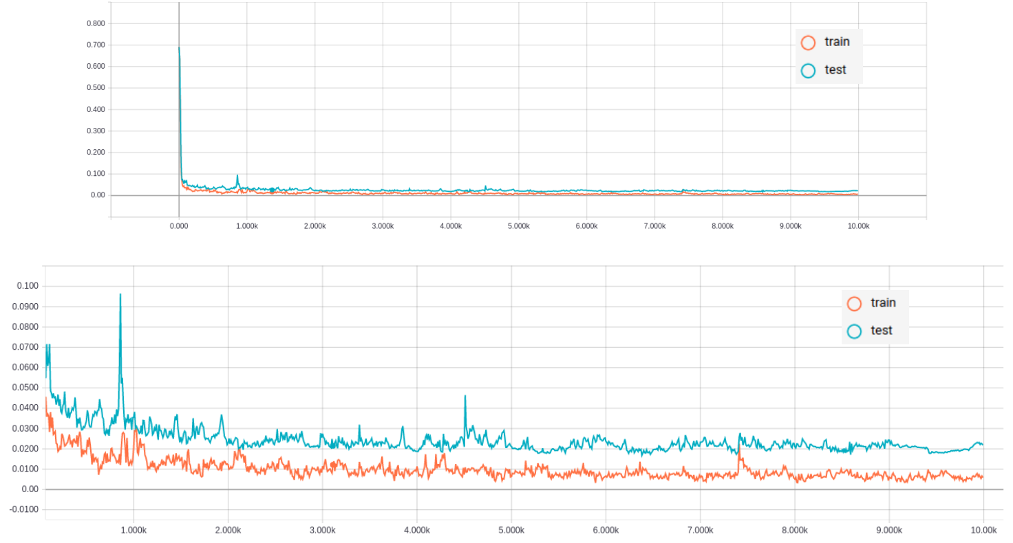
Figure 3.2 Training curve of Model III
Top: training curve; Bottom: zoom in

In figure 3.3, training curves of II and III are plotted in the same graph for comparison. Model II and III have pretty similar performance with respect to cross-entropy loss. The loss on the test set is about 0.23 for both models.

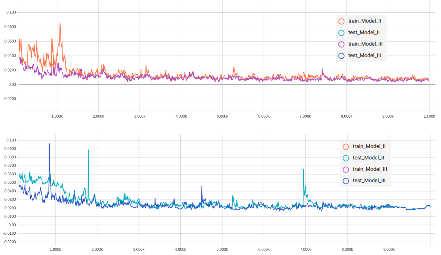
Figure 3.3 Comparison of Model II and Model III
Top: training set; Bottom: test set

3.2 Checkboard artifacts

Visualization analysis is also performed for Model II and III. Refer to figure 3.4 and 3.5 respectively.

According to the visualization result, Model II out-performs Model III a lot with respect to improving checkboard artifacts. It is worth noting that each additional max pooling operation reduces checkboard artifacts in the corresponding deconvolutional feature map.

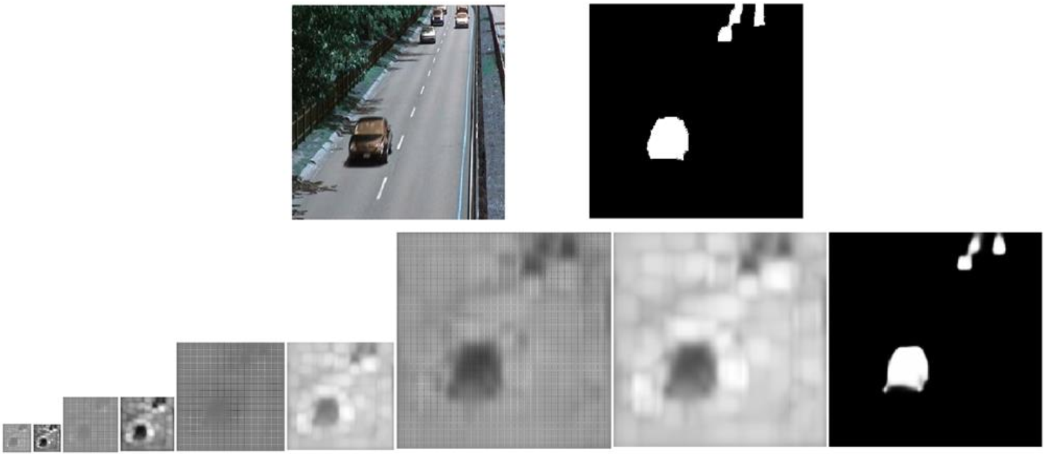
Figure 3.4 (Model II) visualization result of one frame in test set; for each feature map, only the first channel is shown. Top: original image and ground truth; Bottom, from left to right: the output feature of four pairs of deconvolutional+pooling layers, and the final sigmoid activation

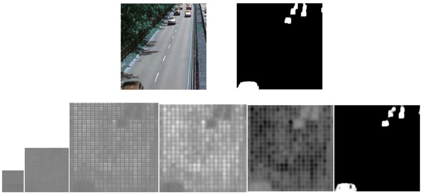
Figure 3.5 (Model III) visualization result of one frame in test set; for each feature map, only the first channel is shown. Top: original image and ground truth; Bottom, from left to right: the output feature of three deconvolutional layers, two convolutional layers, and the final sigmoid activation

3.3 Comparison with classical methods

Now that we’ve got get a satisfactory result on the test, we may still want to know how well does deep learning method generalize? I download a video from the internet, run both SuBSENSE and deep learning method (Model II), and compare the result. Two of the frames are shown in figure 3.6.

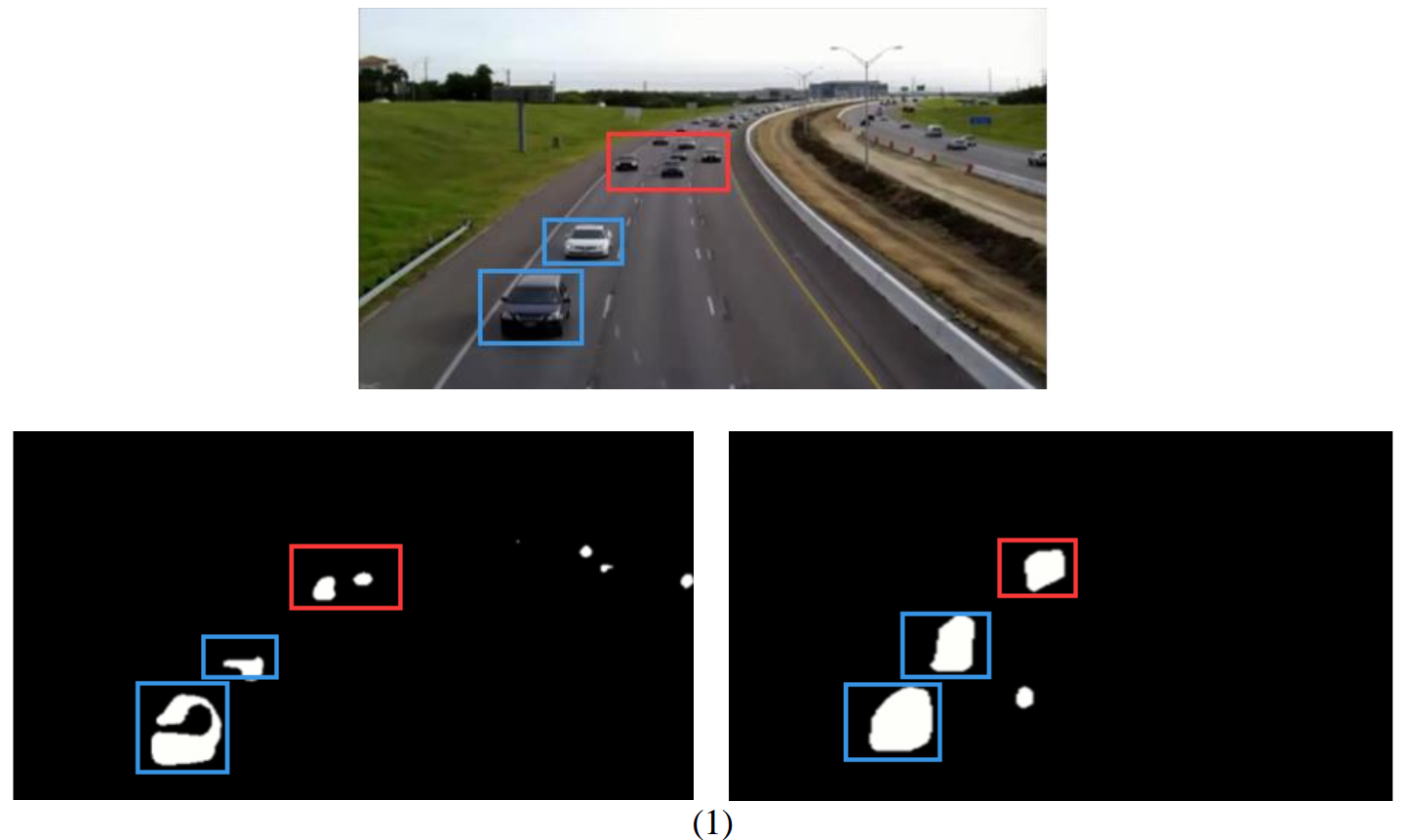
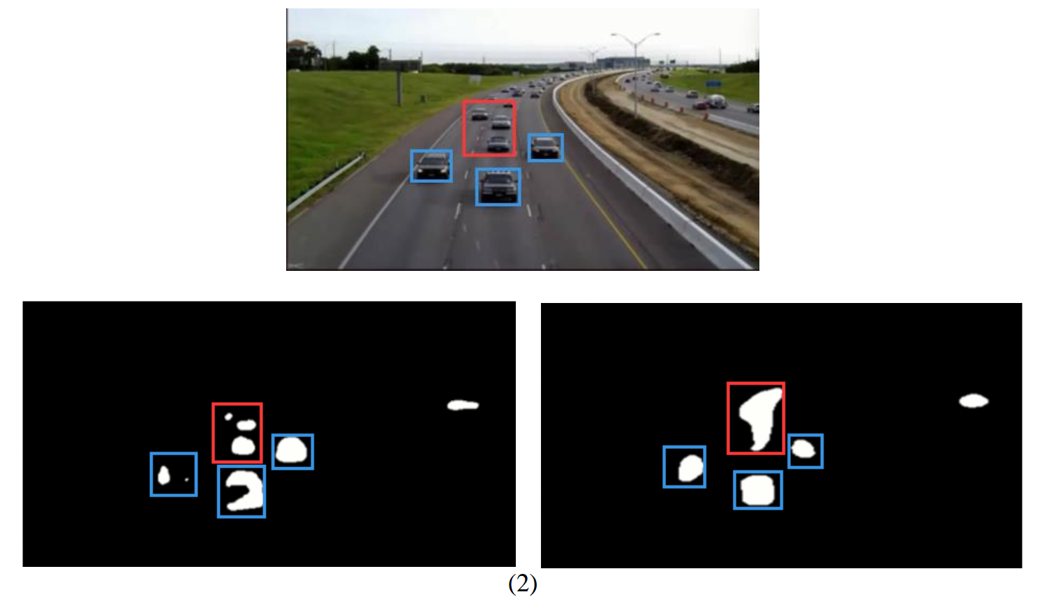
Figure 3.6 background subtraction test on surveillance video
Top: original frame
Bottom left: foreground mask created by SuBSENSE
Bottom right: foreground mask created by Model II

First, let’s focus on the objects highlighted by red rectangles. They are small objects at a relatively longer distance from the camera. With respect to these objects, SuBSENSE out-performs deep learning method. CNN model seems not able to distinguish between small objects.

As for nearer, bigger objects, as is noted by blue rectangles, deep learning method shows its advantage. Foreground masks created by SuBSENSE is often ‘broken’ into parts, and CNN improves this to a large degree.

But why is my model unable to detect small objects? The reason still remains to be figured out.

Reference

[1] Tensorboard: TensorFlow’s Visualization Toolkit
[2] Theano document: Convolution arithmetic tutorial